Damn Cool Algorithms: Levenshtein Automata
Posted by Nick Johnson | Filed under python, tech, coding, damn-cool-algorithms
In a previous Damn Cool Algorithms post, I talked about BK-trees, a clever indexing structure that makes it possible to search for fuzzy matches on a text string based on Levenshtein distance - or any other metric that obeys the triangle inequality. Today, I'm going to describe an alternative approach, which makes it possible to do fuzzy text search in a regular index: Levenshtein automata.
Introduction
The basic insight behind Levenshtein automata is that it's possible to construct a Finite state automaton that recognizes exactly the set of strings within a given Levenshtein distance of a target word. We can then feed in any word, and the automaton will accept or reject it based on whether the Levenshtein distance to the target word is at most the distance specified when we constructed the automaton. Further, due to the nature of FSAs, it will do so in O(n) time with the length of the string being tested. Compare this to the standard Dynamic Programming Levenshtein algorithm, which takes O(mn) time, where m and n are the lengths of the two input words! It's thus immediately apparrent that Levenshtein automaton provide, at a minimum, a faster way for us to check many words against a single target word and maximum distance - not a bad improvement to start with!
Of course, if that were the only benefit of Levenshtein automata, this would be a short article. There's much more to come, but first let's see what a Levenshtein automaton looks like, and how we can build one.
Construction and evaluation
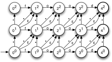
The diagram on the right shows the NFA for a Levenshtein automaton for the word 'food', with maximum edit distance 2. As you can see, it's very regular, and the construction is fairly straightforward. The start state is in the lower left. States are named using a ne style notation, where n is the number of characters consumed so far, and e is the number of errors. Horizontal transitions represent unmodified characters, vertical transitions represent insertions, and the two types of diagonal transitions represent substitutions (the ones marked with a *) and deletions, respectively.
Let's see how we can construct an NFA such as this given an input word and a maximum edit distance. I won't include the source for the NFA class here, since it's fairly standard; for gory details, see the Gist. Here's the relevant function in Python:
def levenshtein_automata(term, k):
  nfa = NFA((0, 0))
  for i, c in enumerate(term):
    for e in range(k + 1):
      # Correct character
      nfa.add_transition((i, e), c, (i + 1, e))
      if e < k:
        # Deletion
        nfa.add_transition((i, e), NFA.ANY, (i, e + 1))
        # Insertion
        nfa.add_transition((i, e), NFA.EPSILON, (i + 1, e + 1))
        # Substitution
        nfa.add_transition((i, e), NFA.ANY, (i + 1, e + 1))
  for e in range(k + 1):
    if e < k:
      nfa.add_transition((len(term), e), NFA.ANY, (len(term), e + 1))
    nfa.add_final_state((len(term), e))
  return nfa
This should be easy to follow; we're basically constructing the transitions you see in the diagram in the most straightforward manner possible, as well as denoting the correct set of final states. State labels are tuples, rather than strings, with the tuples using the same notation we described above.
Because this is an NFA, there can be multiple active states. Between them, these represent the possible interpretations of the string processed so far. For example, consider the active states after consuming the characters 'f' and 'x':
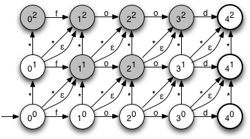
This indicates there are several possible variations that are consistent with the first two characters 'f' and 'x': A single substitution, as in 'fxod', a single insertion, as in 'fxood', two insertions, as in 'fxfood', or a substitution and a deletion, as in 'fxd'. Also included are several redundant hypotheses, such as a deletion and an insertion, also resulting in 'fxod'. As more characters are processed, some of these possibilities will be eliminated, while other new ones will be introduced. If, after consuming all the characters in the word, an accepting (bolded) state is in the set of current states, there's a way to convert the input word into the target word with two or fewer changes, and we know we can accept the word as valid.
Actually evaluating an NFA directly tends to be fairly computationally expensive, due to the presence of multiple active states, and epsilon transitions (that is, transitions that require no input symbol), so the standard practice is to first convert the NFA to a DFA using powerset construction. Using this algorithm, a DFA is constructed in which each state corresponds to a set of active states in the original NFA. We won't go into detail about powerset construction here, since it's tangential to the main topic. Here's an example of a DFA corresponding to the NFA for the input word 'food' with one allowable error:
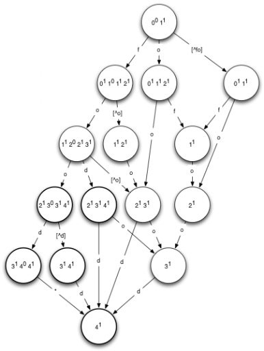
Note that we depicted a DFA for one error, as the DFA corresponding to our NFA above is a bit too complex to fit comfortably in a blog post! The DFA above will accept exactly the words that have an edit distance to the word 'food' of 1 or less. Try it out: pick any word, and trace its path through the DFA. If you end up in a bolded state, the word is valid.
I won't include the source for powerset construction here; it's also in the gist for those who care.
Briefly returning to the issue of runtime efficiency, you may be wondering how efficient Levenshtein DFA construction is. We can construct the NFA in O(kn) time, where k is the edit distance and n is the length of the target word. Conversion to a DFA has a worst case of O(2n) time - which leads to a pretty extreme worst-case of O(2kn) runtime! Not all is doom and gloom, though, for two reasons: First of all, Levenshtein automata won't come anywhere near the 2n worst-case for DFA construction*. Second, some very clever computer scientists have come up with algorithms to construct the DFA directly in O(n) time, [SCHULZ2002FAST] and even a method to skip the DFA construction entirely and use a table-based evaluation method!
Indexing
Now that we've established that it's possible to construct Levenshtein automata, and demonstrated how they work, let's take a look at how we can use them to search an index for fuzzy matches efficiently. The first insight, and the approach many papers [SCHULZ2002FAST] [MIHOV2004FAST] take is to observe that a dictionary - that is, the set of records you want to search - can itself be represented as a DFA. In fact, they're frequently stored as a Trie or a DAWG, both of which can be viewed as special cases of DFAs. Given that both the dictionary and the criteria (the Levenshtein automata) are represented as DFAs, it's then possible to efficiently intersect the two DFAs to find exactly the words in the dictionary that match our criteria, using a very simple procedure that looks something like this:
def intersect(dfa1, dfa2):
  stack = [("", dfa1.start_state, dfa2.start_state)]
  while stack:
    s, state1, state2 = stack.pop()
    for edge in set(dfa1.edges(state1)).intersect(dfa2.edges(state2)):
      state1 = dfa1.next(state1, edge)
      state2 = dfa2.next(state2, edge)
      if state1 and state2:
        s = s + edge
        stack.append((s, state1, state2))
        if dfa1.is_final(state1) and dfa2.is_final(state2):
          yield s
That is, we traverse both DFAs in lockstep, only following edges that both DFAs have in common, and keeping track of the path we've followed so far. Any time both DFAs are in a final state, that word is in the output set, so we output it.
This is all very well if your index is stored as a DFA (or a trie or DAWG), but many indexes aren't: if they're in-memory, they're probably in a sorted list, and if they're on disk, they're probably in a BTree or similar structure. Is there a way we can modify this scheme to work with these sort of indexes, and still provide a speedup on brute-force approaches? It turns out that there is.
The critical insight here is that with our criteria expressed as a DFA, we can, given an input string that doesn't match, find the next string (lexicographically speaking) that does. Intuitively, this is fairly easy to do: we evaluate the input string against the DFA until we cannot proceed further - for example, because there's no valid transition for the next character. Then, we repeatedly follow the edge that has the lexicographically smallest label until we reach a final state. Two special cases apply here: First, on the first transition, we need to follow the lexicographically smallest label greater than character that had no valid transition in the preliminary step. Second, if we reach a state with no valid outwards edge, we should backtrack to the previous state, and try again. This is pretty much the 'wall following' maze solving algorithm, as applied to a DFA.
For an example of this, take a look at the DFA for food(1), above, and consider the input word 'foogle'. We consume the first four characters fine, leaving us in state 3141. The only out edge from here is 'd', while the next character is 'l', so we backtrack one step to the previous state, 21303141. From here, our next character is 'g', and there's an out-edge for 'f', so we take that edge, leaving us in an accepting state (the same state as previously, in fact, but with a different path to it) with the output string 'fooh' - the lexicographically next string in the DFA after 'foogle'.
Here's the Python code for it, as a method on the DFA class. As previously, I haven't included boilerplate for the DFA, which is all here.
  def next_valid_string(self, input):
    state = self.start_state
    stack = []

    # Evaluate the DFA as far as possible
    for i, x in enumerate(input):
      stack.append((input[:i], state, x))
      state = self.next_state(state, x)
      if not state: break
    else:
      stack.append((input[:i+1], state, None))

    if self.is_final(state):
      # Input word is already valid
      return input

    # Perform a 'wall following' search for the lexicographically smallest
    # accepting state.
    while stack:
      path, state, x = stack.pop()
      x = self.find_next_edge(state, x)
      if x:
        path += x
        state = self.next_state(state, x)
        if self.is_final(state):
          return path
        stack.append((path, state, None))
    return None
In the first part of the function, we evaluate the DFA in the normal fashion, keeping a stack of visited states, along with the path so far and the edge we intend to attempt to follow out of them. Then, assuming we didn't find an exact match, we perform the backtracking search we described above, attempting to find the smallest set of transitions we can follow to come to an accepting state. For some caveats about the generality of this function, read on...
Also needed is the utility function find_next_edge, which finds the lexicographically smallest outwards edge from a state that's greater than some given input:
  def find_next_edge(self, s, x):
    if x is None:
      x = u'\0'
    else:
      x = unichr(ord(x) + 1)
    state_transitions = self.transitions.get(s, {})
    if x in state_transitions or s in self.defaults:
      return x
    labels = sorted(state_transitions.keys())
    pos = bisect.bisect_left(labels, x)
    if pos < len(labels):
      return labels[pos]
    return None
With some preprocessing, this could be made substantially more efficient - for example, by pregenerating a mapping from each character to the first outgoing edge greater than it, rather than using binary search to find it in many cases. I once again leave such optimizations as an exercise for the reader.
Now that we have this procedure, we can finally describe how to search the index with it. The algorithm is surprisingly simple:
- Obtain the first element from your index - or alternately, a string you know to be less than any valid string in your index - and call it the 'current' string.
- Feed the current string into the 'DFA successor' algorithm we outlined above, obtaining the 'next' string.
- If the next string is equal to the current string, you have found a match - output it, fetch the next element from the index as the current string, and repeat from step 2.
- If the next string is not equal to the current string, search your index for the first string greater than or equal to the next string. Make this the new current string, and repeat from step 2.
And once again, here's the implementation of this procedure in Python:
def find_all_matches(word, k, lookup_func):
  """Uses lookup_func to find all words within levenshtein distance k of word.

  Args:
    word: The word to look up
    k: Maximum edit distance
    lookup_func: A single argument function that returns the first word in the
      database that is greater than or equal to the input argument.
  Yields:
    Every matching word within levenshtein distance k from the database.
  """
  lev = levenshtein_automata(word, k).to_dfa()
  match = lev.next_valid_string(u'\0')
  while match:
    next = lookup_func(match)
    if not next:
      return
    if match == next:
      yield match
      next = next + u'\0'
    match = lev.next_valid_string(next)
One way of looking at this algorithm is to think of both the Levenshtein DFA and the index as sorted lists, and the procedure above to be similar to App Engine's "zigzag merge join" strategy. We repeatedly look up a string on one side, and use that to jump to the appropriate place on the other side. If there's no matching entry, we use the result of the lookup to jump ahead on the first side, and so forth. The result is that we skip over large numbers of non-matching index entries, as well as large numbers of non-matching Levenshtein strings, saving us the effort of exhaustively enumerating either of them. Hopefully it's apparrent from the description that this procedure has the potential to avoid the need to evaluate either all of the index entries, or all of the candidate Levenshtein strings.
As a side note, it's not true that for all DFAs it's possible to find a lexicographically minimal successor to any string. For example, consider the successor to the string 'a' in the DFA that recognizes the pattern 'a+b'. The answer is that there isn't one: it would have to consist of an infinite number of 'a' characters followed by a single 'b' character! It's possible to make a fairly simple modification to the procedure outlined above such that it returns a string that's guaranteed to be a prefix of the next string recognized by the DFA, which is sufficient for our purposes. Since Levenshtein DFAs are always finite, though, and thus always have a finite length successor (except for the last string, naturally), we leave such an extension as an exercise for the reader. There are potentially interesting applications one could put this approach to, such as indexed regular expression search, which would require this modification.
Testing
First, let's see this in action. We'll define a simple Matcher class, which provides an implementation of the lookup_func required by our find_all_matches function:
class Matcher(object):
  def __init__(self, l):
    self.l = l
    self.probes = 0

  def __call__(self, w):
    self.probes += 1
    pos = bisect.bisect_left(self.l, w)
    if pos < len(self.l):
      return self.l[pos]
    else:
      return None
Note that the only reason we implemented a callable class here is because we want to extract some metrics - specifically, the number of probes made - from the procedure; normally a regular or nested function would be perfectly sufficient. Now, we need a sample dataset. Let's load the web2 dictionary for that:
>>> words = [x.strip().lower().decode('utf-8') for x in open('/usr/share/dict/web2')]
>>> words.sort()
>>> len(words)
234936
We could also use a couple of subsets for testing how things change with scale:
>>> words10 = [x for x in words if random.random() <= 0.1]
>>> words100 = [x for x in words if random.random() <= 0.01]
And here it is in action:
>>> m = Matcher(words)
>>> list(automata.find_all_matches('nice', 1, m))
[u'anice', u'bice', u'dice', u'fice', u'ice', u'mice', u'nace', u'nice', u'niche', u'nick', u'nide', u'niece', u'nife', u'nile', u'nine', u'niue', u'pice', u'rice', u'sice', u'tice', u'unice', u'vice', u'wice']
>>> len(_)
23
>>> m.probes
142
Working perfectly! Finding the 23 fuzzy matches for 'nice' in the dictionary of nearly 235,000 words required 142 probes. Note that if we assume an alphabet of 26 characters, there are 4+26*4+26*5=238 strings within levenshtein distance 1 of 'nice', so we've made a reasonable saving over exhaustively testing all of them. With larger alphabets, longer strings, or larger edit distances, this saving should be more pronounced. It may be instructive to see how the number of probes varies as a function of word length and dictionary size, by testing it with a variety of inputs:
| String length | Max strings | Small dict | Med dict | Full dict |
|---|---|---|---|---|
| 1 | 79 | 47 (59%) | 54 (68%) | 81 (100%) |
| 2 | 132 | 81 (61%) | 103 (78%) | 129 (97%) |
| 3 | 185 | 94 (50%) | 120 (64%) | 147 (79%) |
| 4 | 238 | 94 (39%) | 123 (51%) | 155 (65%) |
| 5 | 291 | 94 (32%) | 124 (43%) | 161 (55%) |
In this table, 'max strings' is the total number of strings within edit distance one of the input string, and the values for small, med, and full dict represent the number of probes required to search the three dictionaries (consisting of 1%, 10% and 100% of the web2 dictionary). All the following rows, at least until 10 characters, required a similar number of probes as row 5. The sample input string used consisted of prefixes of the word 'abracadabra'.
Several observations are immediately apparrent:
- For very short strings and large dictionaries, the number of probes is not much lower - if at all - than the maximum number of valid strings, so there's little saving.
- As the string gets longer, the number of probes required increases significantly slower than the number of potential results, so that at 10 characters, we need only probe 161 of 821 (about 20%) possible results. At commonly encountered word lengths (97% of words in the web2 dictionary are at least 5 characters long), the savings over naively checking every string variation are already significant.
- Although the size of the sample dictionaries differs by an order of magnitude, the number of probes required increases only a little each time. This provides encouraging evidence that this will scale well for very large indexes.
It's also instructive to see how this varies for different edit distance thresholds. Here's the same table, for a max edit distance of 2:
| String length | Max strings | Small dict | Med dict | Full dict |
|---|---|---|---|---|
| 1 | 2054 | 413 (20%) | 843 (41%) | 1531 (75%) |
| 2 | 10428 | 486 (5%) | 1226 (12%) | 2600 (25%) |
| 3 | 24420 | 644 (3%) | 1643 (7%) | 3229 (13%) |
| 4 | 44030 | 646 (1.5%) | 1676 (4%) | 3366 (8%) |
| 5 | 69258 | 648 (0.9%) | 1676 (2%) | 3377 (5%) |
This is also promising: with an edit distance of 2, although we're having to do a lot more probes, it's a much smaller percentage of the number of candidate strings. With a word length of 5 and an edit distance of 2, having to do 3377 probes is definitely far preferable to doing 69,258 (one for every matching string) or 234,936 (one for every word in the dictionary)!
As a quick comparison, a straightforward BK-tree implementation with the same dictionary requires examining 5858 nodes for a string length of 5 and an edit distance of 1 (with the same sample string used above), while the same query with an edit distance of 2 required 58,928 nodes to be examined! Admittedly, many of these nodes are likely to be on the same disk page, if structured properly, but there's still a startling difference in the number of lookups.
One final note: The second paper we referenced in this article, [MIHOV2004FAST] describes a very nifty construction: a universal Levenshtein automata. This is a DFA that determines, in linear time, if any pair of words are within a given fixed Levenshtein distance of each other. Adapting the above scheme to this system is, also, left as an exercise for the reader.
The complete source code for this article can be found here.
* Robust proofs of this hypothesis are welcome.
[SCHULZ2002FAST] Fast string correction with Levenshtein automata
[MIHOV2004FAST] Fast approximate search in large dictionaries
Previous Post Next Post